1、双击打开

2、单击【方方格子】选项卡——【随机重复】——【两区域对比】
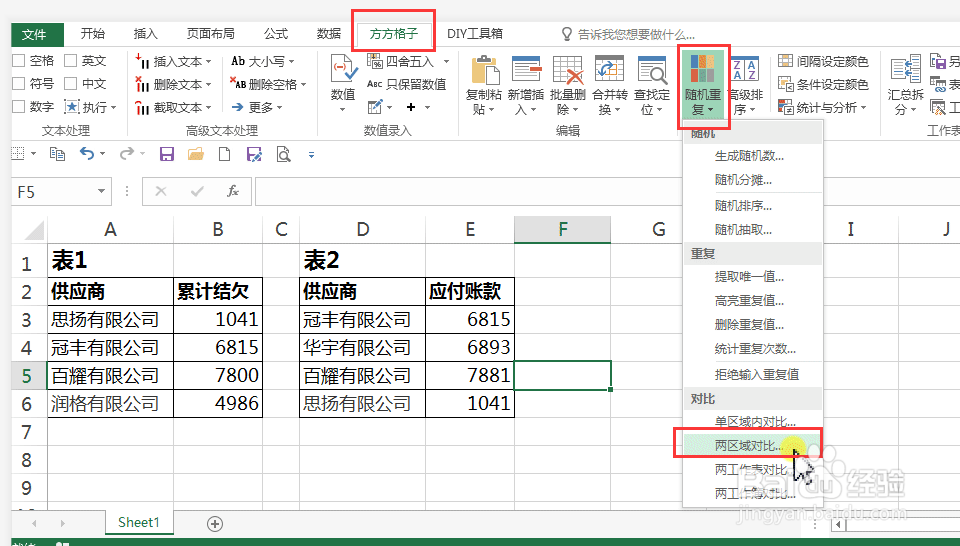
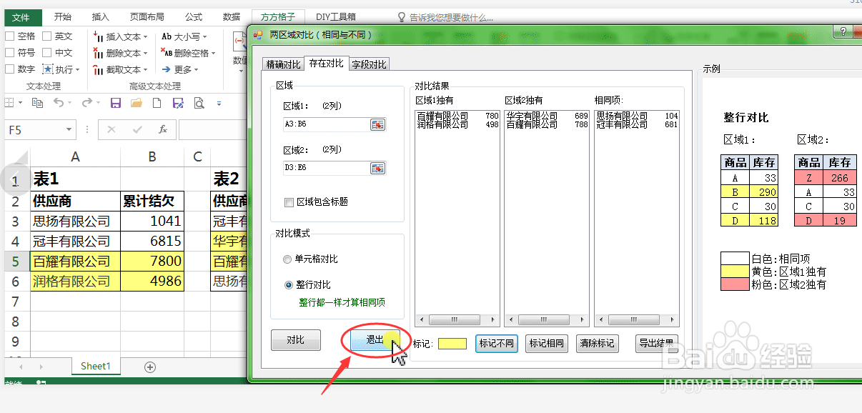
3、在对话框中选择【存在对比】,区域1选择【A3:B6】,区域2选择【D3:E6】,对比模式:【整行对比】,单击【对比】

4、后单击【标记不同】

5、【退出】
6、操作完成,如图。

1、双击打开
2、单击【方方格子】选项卡——【随机重复】——【两区域对比】
3、在对话框中选择【存在对比】,区域1选择【A3:B6】,区域2选择【D3:E6】,对比模式:【整行对比】,单击【对比】
4、后单击【标记不同】
5、【退出】
6、操作完成,如图。