数字信号处理实验三
一﹑实验目的:
通过用Matlab实现信号的分析和表示方法,掌握离散系统分析方法。
二﹑实验要求:
1.了解系统的Matlab描述和转换。
2.掌握分析线性时不变系统的方法,并编程实现。
三﹑实验内容:
1、对给定系统1.H(z)=-0.2z/(+0.8);
(1)求出系统的幅频响应和相频响应;
(2)绘制极零点图;
(3)求出并绘出该系统的单位抽样响应;
(4)令想x(n)=u(n),求出并绘出该系统的单位阶跃响应y(n);
2、y(n)-ay(n-1)=x(n)
y(n)+ay(n-1)=x(n)
其中(a=0.6)
3、H(z)=1/(-z+1);
4、例3-2和例3-5
四﹑实验结果与分析
(Ⅰ)实验程序:
n=512;
b=[0,-0.2];
a=[1,0,0.8];
[h,w]=freqz(b,a,n,'whole')
figure(1)
subplot(2,2,1);
plot(w,abs(h));
xlabel('w');ylabel('·ùƵÏìÓ¦');title('ϵͳÏìÓ¦')
pha=angle(h);
subplot(2,2,2);
plot(w,pha);
xlabel('w');ylabel('ÏàƵÏìÓ¦');
subplot(2,2,3);
zplane(b,a);
subplot(2,2,4)
impz(b,a);
x=stepseq(0,0,50);
y=filter(b,a,x)
n=0:50
figure(2)
stem(y)
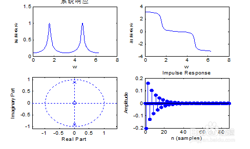
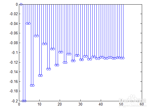
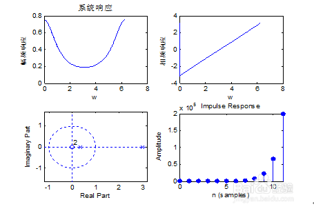
实验结果:
实验分析:
(1)从系统响应看出此响应为带通响应。
(2)从极零点图看出此系统稳定,无法分析是否为因果序列,单位阶跃响应趋于稳定值。
(Ⅱ)
实验程序:
n=[0:10];
b1=1;
a1=[1,-0.6];
b2=1;
a2=[1,0.6];
[h1,w]=freqz(b1,a1);
[h2,w]=freqz(b2,a2);
figure(1)
subplot(2,4,1);
plot(w,abs(h1));
xlabel('w');ylabel('·ùƵÏìÓ¦1');title('ϵͳÏìÓ¦')
subplot(2,4,2);
plot(w,abs(h2));
xlabel('w');ylabel('·ùƵÏìÓ¦2');title('ϵͳÏìÓ¦')
pha1=angle(h1);
subplot(2,4,3);
plot(w,pha1);
xlabel('w');ylabel('ÏàƵÏìÓ¦1');
pha2=angle(h2);
subplot(2,4,4);
plot(w,pha2);
xlabel('w');ylabel('ÏàƵÏìÓ¦2');
subplot(2,4,5);
zplane(b1,a1);title('Á㼫µãͼ1')
subplot(2,4,6);
zplane(b2,a2);title('Á㼫µãͼ2')
subplot(2,4,7)
impz(b1,a1,n);
subplot(2,4,8)
impz(b2,a2,n);
x=stepseq(0,0,10);
y1=filter(b1,a1,x);
y2=filter(b2,a2,x);
figure(2)
subplot(2,1,1)
stem(y1)
xlabel('n');ylabel(' y1(n) ');
subplot(2,1,2)
stem(y2)
xlabel('n');ylabel(' y2(n) ');
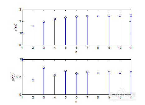
实验结果:
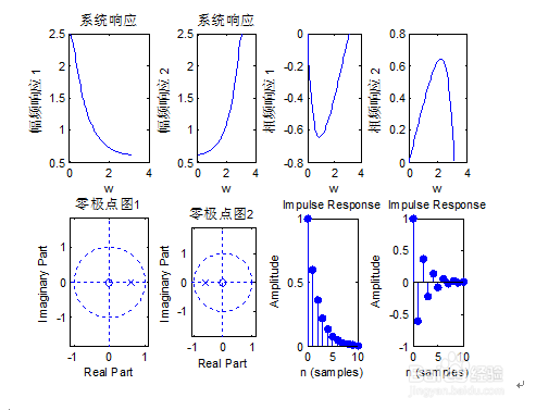
实验分析:
(1)从系统响应看出第一个响应为低通,第二个响应为高通。
(2)从极零点图看出这两个系统稳定,无法分析是否为因果序列,他们的单位阶跃响应趋于稳定值。
(Ⅲ)
实验程序:
n=512;
x=stepseq(0,0,50);
b=1;
a=[1,-10/3,1];
[h,w]=freqz(b,a,n,'whole')
figure(1)
subplot(2,2,1);
plot(w,abs(h));
xlabel('w');ylabel('·ù¶È');title('ϵͳ·ùƵÌØÐÔÇúÏß')
pha=angle(h);
subplot(2,2,2);
plot(w,pha);
title('ϵͳÏàƵÌØÐÔÇúÏß')
xlabel('w');ylabel('Ïàλ');
subplot(2,2,3);
zplane(b,a);
subplot(2,2,4)
impz(b,a);
y=filter(b,a,x)
n=0:50
figure(2)
stem(y)
实验结果:
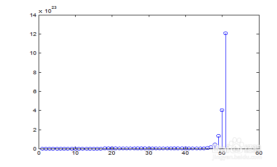
(1)从系统响应看出这个响应为低通。
(2)从极零点图看出这个系统不稳定,单位阶跃响应不趋于稳定值。
(Ⅳ)
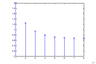
例3-2
n=0:7;
x=(1/4).^n;
Y=[4,10];
xic=filtic(b,a,Y,x)
b=1;
a=[1,-1.5,0.5];
formatlong
y1=filter(b,a,x,xic);
figure(1)
stem(y1);
此系统为稳定系统
例3-5
b=0.15;
a=[1,-0.8];
n=[0:100];
x=2*sin(0.05*pi*n)+0.2*randn(1,101);
imp=[1,zeros(1,100)];
h=impz(b,a,101);
yc=conv(h,x);
y=yc(1:101);
y1=filter(b,a,x);
plot(n,x,'r',n,y1,'b',n,y,'m');
xlabel('n');ylabel('x y yc');title('Timeresponse');
grid ;
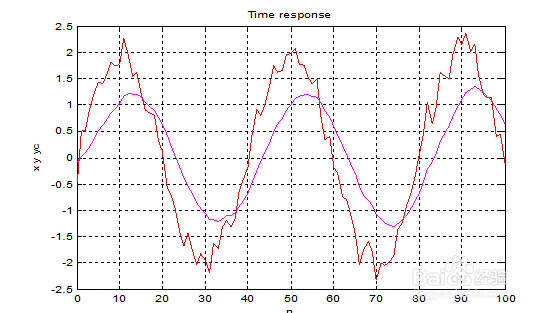
(1)这是滤波器求零状态响应,带尖的图形式输入信号加白噪声信号,平缓的图形式求出的零状态响应,并且两种方法求出的零状态响应图形重合,一种方法是卷积的方法,另一种是滤波器求零状态响应。
五、实验总结
学会了Matlab分析离散系统的方法,做实验时注意数字相乘和字母相乘需要加点,同时注意提前定义所有需要的基本扩展函数,做实验时需要仔细认真!